Class 11 Maths Notes

Chapter 1 Sets

Set
A set is a well-defined collection of objects.

Representation of Sets
There are two methods of representing a set

• Roster or Tabular form In the roster form, we list all the members of the set within braces { } and separate by commas.
• Set-builder form In the set-builder form, we list the property or properties satisfied by all the elements of the sets.

Types of Sets – Class 11 Maths Notes

• Empty Sets: A set which does not contain any element is called an empty set or the void set or null set and it is denoted by {} or Φ.
• Singleton Set: A set consists of a single element, is called a singleton set.
• Finite and infinite Set: A set which consists of a finite number of elements, is called a finite set, otherwise the set is called an infinite set.
• Equal Sets: Two sets A and 6 are said to be equal, if every element of A is also an element of B or vice-versa, i.e. two equal sets will have exactly the same element.
• Equivalent Sets: Two finite sets A and 6 are said to be equal if the number of elements are equal, i.e. n(A) = n(B)

Subset – Class 11 Maths Notes

A set A is said to be a subset of set B if every element of set A belongs to set B. In symbols, we write
A ⊆ B, if x ∈ A ⇒ x ∈ B

Note:

• Every set is o subset of itself.
• The empty set is a subset of every set.
• The total number of subsets of a finite set containing n elements is 2n.

Intervals as Subsets of R
Let a and b be two given real numbers such that a < b, then

• an open interval denoted by (a, b) is the set of real numbers {x : a < x < b}.
• a closed interval denoted by [a, b] is the set of real numbers {x : a ≤ x ≤ b}.
• intervals closed at one end and open at the others are known as semi-open or semi-closed interval and denoted by (a, b] is the set of real numbers {x : a < x ≤ b} or [a, b) is the set of real numbers {x : a ≤ x < b}.

Power Set
The collection of all subsets of a set A is called the power set of A. It is denoted by P(A). If the number of elements in A i.e. n(A) = n, then the number of elements in P(A) = 2n.

Universal Set
A set that contains all sets in a given context is called the universal set.

Venn-Diagrams
Venn diagrams are the diagrams, which represent the relationship between sets. In Venn-diagrams the universal set U is represented by point within a rectangle and its subsets are represented by points in closed curves (usually circles) within the rectangle.

Operations of Sets
Union of sets: The union of two sets A and B, denoted by A ∪ B is the set of all those elements which are either in A or in B or in both A and B. Thus, A ∪ B = {x : x ∈ A or x ∈ B}.

Intersection of sets: The intersection of two sets A and B, denoted by A ∩ B, is the set of all elements which are common to both A and B.
Thus, A ∩ B = {x : x ∈ A and x ∈ B}

Disjoint sets: Two sets Aand Bare said to be disjoint, if A ∩ B = Φ.

Intersecting or Overlapping sets: Two sets A and B are said to be intersecting or overlapping if A ∩ B ≠ Φ

Difference of sets: For any sets A and B, their difference (A – B) is defined as a set of elements, which belong to A but not to B.
Thus, A – B = {x : x ∈ A and x ∉ B}
also, B – A = {x : x ∈ B and x ∉ A}

Complement of a set: Let U be the universal set and A is a subset of U. Then, the complement of A is the set of all elements of U which are not the element of A.
Thus, A’ = U – A = {x : x ∈ U and x ∉ A}

Some Properties of Complement of Sets

• A ∪ A’ = ∪
• A ∩ A’ = Φ
• ∪’ = Φ
• Φ’ = ∪
• (A’)’ = A

Symmetric difference of two sets: For any set A and B, their symmetric difference (A – B) ∪ (B – A)
(A – B) ∪ (B – A) defined as set of elements which do not belong to both A and B.
It is denoted by A ∆ B.
Thus, A ∆ B = (A – B) ∪ (B – A) = {x : x ∉ A ∩ B}.

Laws of Algebra of Sets – Class 11 Maths Notes

Idempotent Laws: For any set A, we have

• A ∪ A = A
• A ∩ A = A

Identity Laws: For any set A, we have

• A ∪ Φ = A
• A ∩ U = A

Commutative Laws: For any two sets A and B, we have

• A ∪ B = B ∪ A
• A ∩ B = B ∩ A

Associative Laws: For any three sets A, B and C, we have

• A ∪ (B ∪ C) = (A ∪ B) ∪ C
• A ∩ (B ∩ C) = (A ∩ B) ∩ C

Distributive Laws: If A, B and Care three sets, then

• A ∪ (B ∩ C) = (A ∪ B) ∩ (A ∪ C)
• A ∩ (B ∪ C) = (A ∩ B) ∪ (A ∩ C)

De-Morgan’s Laws: If A and B are two sets, then

• (A ∪ B)’ = A’ ∩ B’
• (A ∩ B)’ = A’ ∪ B’

Formulae to Solve Practical Problems on Union and Intersection of Two Sets
Let A, B and C be any three finite sets, then

• n(A ∪ B) = n(A) + n (B) – n(A ∩ B)
• If (A ∩ B) = Φ, then n (A ∪ B) = n(A) + n(B)
• n(A – B) = n(A) – n(A ∩ B)
• n(A ∪ B ∪ C) = n(A) + n(B) + n(C) – n(A ∩ B) – n(B ∩ C) – n(A ∩ C) + n(A ∩ B ∩ C)

Chapter 2 Relations and Functions

Ordered Pair
An ordered pair consists of two objects or elements in a given fixed order.

Equality of Two Ordered Pairs
Two ordered pairs (a, b) and (c, d) are equal if a = c and b = d.

Cartesian Product of Two Sets
For any two non-empty sets A and B, the set of all ordered pairs (a, b) where a ∈ A and b ∈ B is called the cartesian product of sets A and B and is denoted by A × B.
Thus, A × B = {(a, b) : a ∈ A and b ∈ B}
If A = Φ or B = Φ, then we define A × B = Φ

Note:

• A × B ≠ B × A
• If n(A) = m and n(B) = n, then n(A × B) = mn and n(B × A) = mn
• If atieast one of A and B is infinite, then (A × B) is infinite and (B × A) is infinite.

Relations
A relation R from a non-empty set A to a non-empty set B is a subset of the cartesian product set A × B. The subset is derived by describing a relationship between the first element and the second element of the ordered pairs in A × B.
The set of all first elements in a relation R is called the domain of the relation B, and the set of all second elements called images is called the range of R.

Note:

• A relation may be represented either by the Roster form or by the set of builder form, or by an arrow diagram which is a visual representation of relation.
• If n(A) = m, n(B) = n, then n(A × B) = mn and the total number of possible relations from set A to set B = 2mn

Inverse of Relation
For any two non-empty sets A and B. Let R be a relation from a set A to a set B. Then, the inverse of relation R, denoted by R-1 is a relation from B to A and it is defined by
R-1 ={(b, a) : (a, b) ∈ R}
Domain of R = Range of R-1 and
Range of R = Domain of R-1.

Functions
A relation f from a set A to set B is said to be function, if every element of set A has one and only image in set B.
In other words, a function f is a relation such that no two pairs in the relation have the first element.

Real-Valued Function
A function f : A → B is called a real-valued function if B is a subset of R (set of all real numbers). If A and B both are subsets of R, then f is called a real function.

Some Specific Types of Functions
Identity function: The function f : R → R defined by f(x) = x for each x ∈ R is called identity function.
Domain of f = R; Range of f = R

Constant function: The function f : R → R defined by f(x) = C, x ∈ R, where C is a constant ∈ R, is called a constant function.
Domain of f = R; Range of f = C

Polynomial function: A real valued function f : R → R defined by f(x) = a0 + a1x + a2x2+…+ anxn, where n ∈ N and a0, a1, a2,…….. an ∈ R for each x ∈ R, is called polynomial function.

Rational function: These are the real function of type f(x)g(x), where f(x)and g(x)are polynomial functions of x defined in a domain, where g(x) ≠ 0.

The modulus function: The real function f : R → R defined by f(x) = |x|
or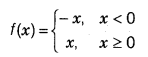

for all values of x ∈ R is called the modulus function.
Domaim of f = R
Range of f = R+ U {0} i.e. [0, ∞)

Signum function: The real function f : R → R defined
by f(x) = |x|x, x ≠ 0 and 0, if x = 0
or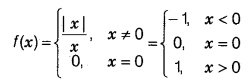

is called the signum function.
Domain of f = R; Range of f = {-1, 0, 1}

Greatest integer function: The real function f : R → R defined by f (x) = {x}, x ∈ R assumes that the values of the greatest integer less than or equal to x, is called the greatest integer function.
Domain of f = R; Range of f = Integer

Fractional part function: The real function f : R → R defined by f(x) = {x}, x ∈ R is called the fractional part function.
f(x) = {x} = x – [x] for all x ∈R
Domain of f = R; Range of f = [0, 1)

Algebra of Real Functions
Addition of two real functions: Let f : X → R and g : X → R be any two real functions, where X ∈ R. Then, we define (f + g) : X → R by
{f + g) (x) = f(x) + g(x), for all x ∈ X.

Subtraction of a real function from another: Let f : X → R and g : X → R be any two real functions, where X ⊆ R. Then, we define (f – g) : X → R by (f – g) (x) = f (x) – g(x), for all x ∈ X

Multiplication by a scalar: Let f : X → R be a real function and K be any scalar belonging to R. Then, the product of Kf is function from X to R defined by (Kf)(x) = Kf(x) for all x ∈ X.

Multiplication of two real functions: Let f : X → R and g : X → R be any two real functions, where X ⊆ R. Then, product of these two functions i.e. f.g : X → R is defined by (fg) x = f(x) . g(x) ∀ x ∈ X.

Quotient of two real functions: Let f and g be two real functions defined from X → R. The quotient of f by g denoted by 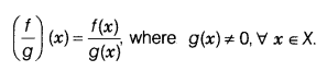fg is a function defined from X → R as

Chapter 3 Trigonometric Functions

Angle
Angle is a measure of rotation of a given ray about its initial point. The original ray is called the initial side and the final position of ray after rotation is called terminal side of the angle. The point of rotation is called vertex. If the direction of rotation is anti-clockwise, the angle is said to be positive and if the direction of rotation is clockwise, then the angle is negative.

Measuring Angles
There are two systems of measuring angles
Sexagesimal system (degree measure): If a rotation from the initial side to terminal side is (1360)th of a revolution, the angle is said to have a measure of one degree, written as 1°.
One sixtieth of a degree is called a minute, written as 1′ and one-sixtieth of a minute is called a second, written as 1″
Thus, 1° = 60′ and 1′ = 60″

Circular system (radian measure): A radian is an angle subtended at the centre of a circle by an arc, whose length is equal to the radius of the circle. We denote 1 radian by 1°.

Relation Between Radian and Degree
We know that a complete circle subtends at its centre an angle whose measure is 2π radians as well as 360°.
2π radian = 360°.
Hence, π radian = 180°
or 1 radian = 57° 16′ 21″ (approx)
1 degree = 0.01746 radian

Six Fundamental Trigonometric Identities

• sinx = 1cosecx
• cos x = 1secx
• tan x = 1cotx
• sin2 x + cos2 x = 1
• 1 + tan2x = sec2 x
• 1 + cot2 x = cosec2 x

Trigonometric Functions – Class 11 Maths Notes

Trigonometric ratios are defined for acute angles as the ratio of the sides of a right angled triangle. The extension of trigonometric ratios to any angle in terms of radian measure (real number) are called trigonometric function. The signs of trigonometric function in different quadrants have been given in following table.

	I	II	III	IV
Sin x	+	+	–	–
Cos x	+	–	–	+
Tan x	+	–	+	–
Cosec x	+	+	–	–
Sec x	+	–	–	+
Cot x	+	–	+	–

Domain and Range of Trigonometric Functions

 

Functions	Domain	Range
Sine	R	[-1, 1]
Cos	R	[-1, 1]
Tan	R – {(2n + 1) π2 : n ∈ Z	R
Cot	R – {nπ: n ∈ Z}	R
Sec	R – {(2n + 1) π2 : n ∈ Z	R – (-1, 1)
Cosec	R – {nπ: n ∈ Z}	R – (-1, 1)

Sine, Cosine, and Tangent of Some Angles Less Than 90°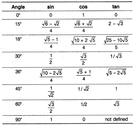

Allied or Related Angles
The angles nπ2±θ are called allied or related angle and θ ± n × (2π) are called coterminal angles. For general reduction, we have following rules, the value of trigonometric function for (nπ2±θ) is numerically equal to

• the value of the same function, if n is an even integer with the algebraic sign of the function as per the quadrant in which angle lies.
• the corresponding co-function of θ, if n is an odd integer with the algebraic sign of the function for the quadrant in which it lies, here sine and cosine, tan and cot, sec and cosec are cofunctions of each other.

Functions of Negative Angles

For any acute angle of θ.
We have,

• sin(-θ) = – sinθ
• cos (-θ) = cosθ
• tan (-θ) = – tanθ
• cot (-θ) = – cotθ
• sec (-θ) = secθ
• cosec (-θ) = – cosecθ

Some Formulae Regarding Compound Angles

An angle made up of the sum or difference of two or more angles is called compound angles. The basic results in direction are called trigonometric identities as given below:
(i) sin (x + y) = sin x cos y + cos x sin y
(ii) sin (x – y) = sin x cos y – cos x sin y
(iii) cos (x + y) = cos x cos y – sin x sin y
(iv) cos (x – y) = cos x cos y + sin x sin y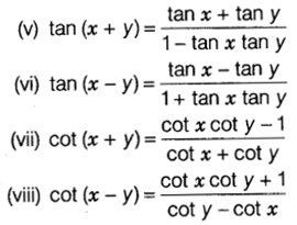

(ix) sin(x + y) sin (x – y) = sin2 x – sin2 y = cos2 y – cos2 x
(x) cos (x + y) cos (x – y) = cos2 x – sin2 y = cos2 y – sin2 x

Transformation Formulae

• 2 sin x cos y = sin (x + y) + sin (x – y)
• 2 cos x sin y = sin (x + y) – sin (x – y)
• 2 cos x cos y = cos (x + y) + cos (x – y)
• 2 sin x sin y = cos (x – y) – cos (x + y)
• sin x + sin y = 2 sin(x+y2) cos(x−y2)
• sin x – sin y = 2 cos(x+y2) sin(x−y2)
• cos x + cos y = 2 cos(x+y2) cos(x−y2)
• cos x – cos y = -2 sin(x+y2) sin(x−y2)

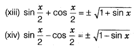
Trigonometric Ratios of Multiple Angles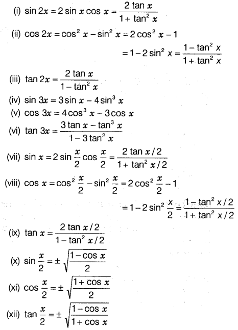

Product of Trigonometric Ratios

• sin x sin (60° – x) sin (60° + x) = 14 sin 3x
• cos x cos (60° – x) cos (60° + x) = 14 cos 3x
• tan x tan (60° – x) tan (60° + x) = tan 3x
• cos 36° cos 72° = 14
• cos x . cos 2x . cos 22x . cos 23x … cos 2n-1 = sin2nx2nsinx

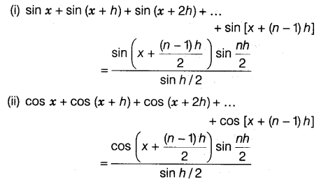
Sum of Trigonometric Ratio, if Angles are in A.P.

Trigonometric Equations
Equation which involves trigonometric functions of unknown angles is known as the trigonometric equation.

Solution of a Trigonometric Equation
A solution of a trigonometric equation is the value of the unknown angle that satisfies the equation.
A trigonometric equation may have an infinite number of solutions.

Principal Solution
The solutions of a trigonometric equation for which 0 ≤ x ≤ 2π are called principal solutions.

General Solutions
A solution of a trigonometric equation, involving ‘n’ which gives all solution of a trigonometric equation is called the general solutions.

General Solutions of Trigonometric Equation

• sin x = 0 ⇔ x = nπ, n ∈ Z
• cos x = 0 ⇔ x = (2n + 1) π2 , n ∈ Z
• tan x = 0 ⇔ x = nπ, n ∈ Z
• sin x = sin y ⇔ x = nπ + (-1)n y, n ∈ Z
• cos x = cos y ⇔ x = 2nπ ± y, n ∈ Z
• tan x = tan y ⇔ x = nπ ± y, n ∈ Z
• sin2 x = sin2 y ⇔ x = nπ ± y, n ∈ Z
• cos2 x = cos2 y ⇔ x = nπ ± y, n ∈ Z
• tan2 x = tan2 y ⇔ x = nπ ± y, n ∈ Z

Basic Rules of Triangle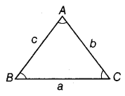

In a triangle ABC, the angles are denoted by capital letters A, B and C and the lengths of sides of opposite to these angles are denoted by small letters a, b and c, respectively.
Sine Rule
sinAa=sinBb=sinCc

Cosine Rule
a2 = b2 + c2 – 2bc cos A
b2 = c2 + a2 – 2ac cos B
c2 = a2 + b2 – 2ab cos C

Projection Rule
a = b cos C + c cos B
b = c cos A + a cos C
c = a cos B + b cos A

 Chapter 4 Principle of Mathematical Induction

Principle of Mathematical Induction
Mathematical induction is one of the techniques, which can be used to prove a variety of mathematical statements which are formulated in terms of n, where n is a positive integer.

Let P(n) be given statement involving the natural number n such that
(i) The statement is true for n = 1, i.e. P(1) is true.
(ii) If the statement is true for n = k (where k is a particular but arbitrary natural number), then the statement is also true for n = k + 1 i.e. truth of P(k) implies that the truth of P(k + 1). Then, P(n) is true for all natural numbers n.

Chapter 5 Complex Numbers and Quadratic Equations

Imaginary Numbers
The square root of a negative real number is called an imaginary number, e.g. √-2, √-5 etc.
The quantity √-1 is an imaginary unit and it is denoted by ‘i’ called Iota.

Integral Power of IOTA (i)
i = √-1, i2 = -1, i3 = -i, i4 = 1
So, i4n+1 = i, i4n+2 = -1, i4n+3 = -i, i4n = 1

Note:

• For any two real numbers a and b, the result √a × √b : √ab is true only, when atleast one of the given numbers i.e. either zero or positive.
  √-a × √-b ≠ √ab
  So, i2 = √-1 × √-1 ≠ 1
• ‘i’ is neither positive, zero nor negative.
• in + in+1 + in+2 + in+3 = 0

Complex Number
A number of the form x + iy, where x and y are real numbers, is called a complex number, x is called real part and y is called imaginary part of the complex number i.e. Re(Z) = x and Im(Z) = y.

Purely Real and Purely Imaginary Complex Number
A complex number Z = x + iy is a purely real if its imaginary part is 0, i.e. Im(z) = 0 and purely imaginary if its real part is 0 i.e. Re (z) = 0.

Equality of Complex Number
Two complex numbers z1 = x1 + iy1 and z2 = x2 + iy2 are equal, iff x1 = x2 and y1 = y2 i.e. Re(z1) = Re(z2) and Im(z1) = Im(z2)
Note: Order relation “greater than’’ and “less than” are not defined for complex number.

Algebra of Complex Numbers
Addition of complex numbers
Let z1 = x1 + iy1 and z2 = x2 + iy2 be any two complex numbers, then their sum defined as
z1 + z2 = (x1 + iy1) + (x2 + iy2) = (x1 + x2) + i (y1 + y2)

Properties of Addition

• Commutative: z1 + z2 = z2 + z1
• Associative: z1 + (z2 + z3) = (z1 + z2) + z3
• Additive identity z + 0 = z = 0 + z
  Here, 0 is additive identity.

Subtraction of complex numbers
Let z1 = (x1 + iy1) and z2 = (x2 + iy2) be any two complex numbers, then their difference is defined as
z1 – z2 = (x1 + iy1) – (x2 + iy2) = (x1 – x2) + i(y1 – y2)

Multiplication of complex numbers
Let z1 = (x1 + iy1) and z2 = (x2 + iy2) be any two complex numbers, then their multiplication is defined as
z1z2 = (x1 + iy1) (x2 + iy2) = (x1x2 – y1y2) + i (x1y2 + x2y1)

Properties of Multiplication

• Commutative: z1z2 = z2z1
• Associative: z1(z2z3) = (z1z2)z3
• Multiplicative identity: z . 1 = z = 1 . z
  Here, 1 is multiplicative identity of an element z.
• Multiplicative inverse: For every non-zero complex number z, there exists a complex number z1 such that z . z1 = 1 = z1 . z
• Distributive law: z1(z2 + z3) = z1z2 + z1z3

Division of Complex Numbers
Let z1 = x1 + iy1 and z2 = x2 + iy2 be any two complex numbers, then their division is defined as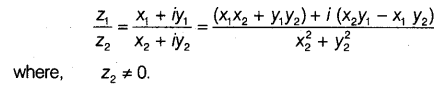

Conjugate of Complex Number
Let z = x + iy, if ‘i’ is replaced by (-i), then said to be conjugate of the complex number z and it is denoted by z¯, i.e. z¯ = x – iy

Properties of Conjugate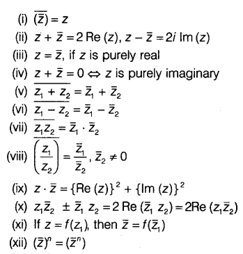

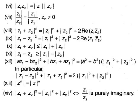
Modulus of a Complex Number
Let z = x + iy be a complex number. Then, the positive square root of the sum of square of real part and square of imaginary part is called modulus (absolute values) of z and it is denoted by |z| i.e. |z| = x2+y2−−−−−−√
It represents a distance of z from origin in the set of complex number c, the order relation is not defined
i.e. z1 > z2 or z1 < z2 has no meaning but |z1| > |z2| or |z1|<|z2| has got its meaning, since |z1| and |z2| are real numbers.

Properties of Modulus of a Complex number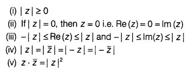

Argand Plane
Any complex number z = x + iy can be represented geometrically by a point (x, y) in a plane, called argand plane or gaussian plane. A purely number x, i.e. (x + 0i) is represented by the point (x, 0) on X-axis. Therefore, X-axis is called real axis. A purely imaginary number iy i.e. (0 + iy) is represented by the point (0, y) on the y-axis. Therefore, the y-axis is called the imaginary axis.

Argument of a complex Number
The angle made by line joining point z to the origin, with the positive direction of X-axis in an anti-clockwise sense is called argument or amplitude of complex number. It is denoted by the symbol arg(z) or amp(z).
arg(z) = θ = tan-1(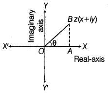yx)

Argument of z is not unique, general value of the argument of z is 2nπ + θ, but arg(0) is not defined. The unique value of θ such that -π < θ ≤ π is called the principal value of the amplitude or principal argument.

Principal Value of Argument

• if x > 0 and y > 0, then arg(z) = θ
• if x < 0 and y > 0, then arg(z) = π – θ
• if x < 0 and y < 0, then arg(z) = -(π – θ)
• if x > 0 and y < 0, then arg(z) = -θ

Polar Form of a Complex Number
If z = x + iy is a complex number, then z can be written as z = |z| (cosθ + isinθ), where θ = arg(z). This is called polar form. If the general value of the argument is θ, then the polar form of z is z = |z| [cos (2nπ + θ) + isin(2nπ + θ)], where n is an integer.

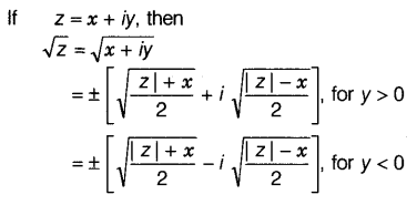
Square Root of a Complex Number

Solution of a Quadratic Equation
The equation ax2 + bx + c = 0, where a, b and c are numbers (real or complex, a ≠ 0) is called the general quadratic equation in variable x. The values of the variable satisfying the given equation are called roots of the equation.

The quadratic equation ax2 + bx + c = 0 with real coefficients has two roots given by −b+√D2a and −b−√D2a, where D = b2 – 4ac, called the discriminant of the equation.

Note:
(i) When D = 0, roots ore real and equal. When D > 0 roots are real and unequal. Further If a,b, c ∈ Q and D is perfect square, then the roots of quadratic equation are real and unequal and if a, b, c ∈ Q and D is not perfect square, then the roots are irrational and occur in pair. When D < 0, roots of the equation are non real (or complex).

(ii) Let α, β be the roots of quadratic equation ax2 + bx + c = 0, then sum of roots α + β = −ba and the product of roots αβ = ca.

Chapter 6 Linear Inequalities

Inequation
A statement involving variables and the sign of inequality viz. >, <, ≥ or ≤ is called an inequation or an inequality.

Numerical Inequalities
Inequalities which do not contain any variable is called numerical inequalities, e.g. 3 < 7, 2 ≥ -1, etc. Literal Inequalities Inequalities which contains variables are called literal inequalities e.g. x – y > 0, x > 5, etc.

Linear Inequation of One Variable
Let a be non-zero real number and x be a variable. Then, inequalities of the form ax + b > 0, ax + b < 0, ax + b ≥ 0 and ax + b ≤ 0 are known as linear inequalities in one variable.

Linear Inequation of Two Variables
Let a, b be non-zero real numbers and x, y be variables. Then, inequation of the form ax + by < c, ax + by > c, ax + by ≤ c and ax + by ≥ c are known as linear inequalities in two variables x and y.

Solution of an Inequality
The value(s) of the variable(s) which makes the inequality a true statement is called its solutions. The set of all solutions of an inequality is called the solution set of the inequality.

Solving Linear Inequations in One Variable
Same number may be added (or subtracted) to both sides of an inequation without changing the sign of inequality.

Both sides of an inequation can be multiplied (or divided) by the same positive real number without changing the sign of inequality. However, the sign of inequality is reversed when both sides of an inequation are multiplied or divided by a negative number.

Representation of Solution of Linear Inequality in One Variable on a Number Line
To represent the solution of a linear inequality in one variable on a number line. We use the following algorithm.

If the inequality involves ‘>’ or ‘<‘ we draw an open circle (O) on the number line, which indicates that the number corresponding to the open circle is not included in the solution set.

If the inequality involves ‘≥’ or ‘≤’ we draw a dark circle (•) on the number line, which indicates the number corresponding to the dark circle is included in the solution set.

Graphical Representation of the Solution of Linear Inequality in One or Two Variables
To represent the solution of linear inequality in one or two variables graphically in a plane, we use the following algorithm.

If the inequality involves ‘<’ or ‘>’, we draw the graph of the line as dotted line to indicate that the points on the line are not included from the solution sets.

If the inequality involves ‘≥’ or ‘≤’, we draw the graph of the line as a dark line to indicate the points on the line is included from the solution sets.

Solution of a linear inequality in one variable can be represented on number line as well as in the plane but the solution of a linear inequality in two variables of the type ax + by > c, ax + by ≥ c,ax + by < c or ax + by ≤ c (a ≠ 0, b ≠ 0) can be represented in the plane only.

Two or more inequalities taken together comprise a system of inequalities and the solution of the system of inequalities are the solution common to all the inequalities comprising the system.

Chapter 7 Permutations and Combinations

Fundamental Principles of Counting
Multiplication Principle: Suppose an operation A can be performed in m ways and associated with each way of performing of A, another operation B can be performed in n ways, then total number of performance of two operations in the given order is mxn ways. This can be extended to any finite number of operations.

Addition Principle: If an operation A can be performed in m ways and another operation S, which is independent of A, can be performed in n ways, then A and B can performed in (m + n) ways. This can be extended to any finite number of exclusive events.

Factorial
The continued product of first n natural number is called factorial ‘n’.
It is denoted by n! or n! = n(n – 1)(n – 2)… 3 × 2 × 1 and 0! = 1! = 1

Permutation
Each of the different arrangement which can be made by taking some or all of a number of objects is called permutation.

Permutation of n different objects
The number of arranging of n objects taking all at a time, denoted by nPn, is given by nPn = n!
The number of an arrangement of n objects taken r at a time, where 0 < r ≤ n, denoted by nPr is given by
nPr = n!(n−r)!

Properties of Permutation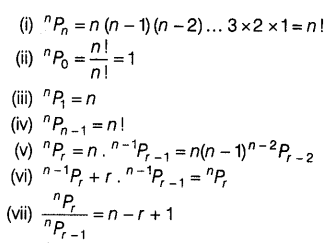

Important Results on Permutation
The number of permutation of n things taken r at a time, when repetition of object is allowed is nr.

The number of permutation of n objects of which p1 are of one kind, p2 are of second kind,… pk are of kth kind such that p1 + p2 + p3 + … + pk = n is n!p1!p2!p3!…..pk!

Number of permutation of n different objects taken r at a time,
When a particular object is to be included in each arrangement is r. n-1Pr-1

When a particular object is always excluded, then number of arrangements = n-1Pr.

Number of permutations of n different objects taken all at a time when m specified objects always come together is m! (n – m + 1)!.

Number of permutation of n different objects taken all at a time when m specified objects never come together is n! – m! (n – m + 1)!.

Combinations
Each of the different selections made by taking some or all of a number of objects irrespective of their arrangements is called combinations. The number of selection of r objects from; the given n objects is denoted by nCr, and is given by
nCr = n!r!(n−r)!

Properties of Combinations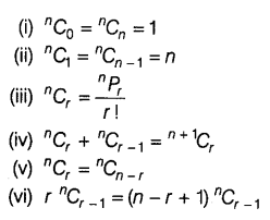

Chapter 8 Binomial Theorem

Binomial Expression
An expression consisting of two terms, connected by + or – sign is called binomial expression.

Binomial Theorem
If a and b are real numbers and n is a positive integer, then

The general term of (r + 1)th term in the expression is given by
Tr+1 = nCr an-r br

Some Important Observations from the Binomial Theorem
The total number of terms in the binomial expansion of (a + b)n is n + 1.

The sum of the indices of a and b in each term is n.

The coefficient of terms equidistant from the beginning and the end are equal. These coefficients are known as the binomial coefficient and
nCr = nCn-r, r = 0, 1, 2, 3,…, n

The values of the binomial coefficient steadily increase to a maximum and then steadily decrease.

The coefficient of xr in the expansion of (1 + x)n is nCr.

In the binomial expansion (a + b)n, the rth term from the end is (n – r + 2)th term from the beginning.

Middle Term in the Expansion of (a + b)n
If n is even, then in the expansion of (a + b)n, the middle term is (n2 + 1) th term.

If n is odd, then in the expansion of (a + b)n, the middle terms are (n+12)th term and (n+32)th term.

Chapter 9 Sequences and Series

Sequence
A succession of numbers arranged in a definite order according to a given certain rule is called sequence. A sequence is either finite or infinite depending upon the number of terms in a sequence.

Series
If a1, a2, a3,…… an is a sequence, then the expression a1 + a2 + a3 + a4 + … + an is called series.

Progression
A sequence whose terms follow certain patterns are more often called progression.

Arithmetic Progression (AP)
A sequence in which the difference of two consecutive terms is constant, is called Arithmetic progression (AP).

Properties of Arithmetic Progression (AP)
If a sequence is an A.P. then its nth term is a linear expression in n i.e. its nth term is given by An + B, where A and S are constant and A is common difference.

nth term of an AP : If a is the first term, d is common difference and l is the last term of an AP then

• nth term is given by an = a + (n – 1)d.
• nth term of an AP from the last term is a’n =an – (n – 1)d.
• an + a’n = constant
• Common difference of an AP i.e. d = an – an-1,∀ n > 1.

If a constant is added or subtracted from each term of an AR then the resulting sequence is an AP with same common difference.

If each term of an AP is multiplied or divided by a non-zero constant, then the resulting sequence is also an AP.

If a, b and c are three consecutive terms of an A.P then 2b = a + c.

Any three terms of an AP can be taken as (a – d), a, (a + d) and any four terms of an AP can be taken as (a – 3d), (a – d), (a + d), (a + 3d)

Sum of n Terms of an AP
Sum of n terms of an AP is given by
Sn = n2 [2a + (n – 1)d] = n2 (a1+ an)

A sequence is an AP If the sum of n terms is of the form An2 + Bn, where A and B are constant and A = half of common difference i.e. 2A = d.

an =Sn – Sn-1

Arithmetic Mean
If a, A and b are in A.P then A = a+b2 is called the arithmetic mean of a and b.

If a1, a2, a3,……an are n numbers, then their arithmetic mean is given by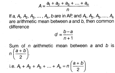

Geometric Progression (GP)
A sequence in which the ratio of two consecutive terms is constant is called geometric progression. The constant ratio is called common ratio(r).
i.e. r = an+1an, ∀ n > 1

Properties of Geometric Progression
If a is the first term and r is the common ratio, then the general term or nth term of GP is an =arn-1

nth term of a GP from the end is a’n = 1rn−1, l = last term

If all the terms of GP be multiplied or divided by same non-zero constant, then the resulting sequence is a GP with the same common ratio.

The reciprocal terms of a given GP form a GP.

If each term of a GP be raised to some power, the resulting sequence also forms a GP

If a, b and c are three consecutive terms of a GP then b2 = ac.

Any three terms can be taken in GP as ar, a and ar and any four terms can be taken in GP as ar3, ar, ar and ar3.

Sum of n Terms of a G.P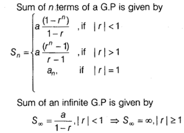

Geometric Mean (GM)
If a, G and b are in GR then G is called the geometric mean of a and b and is given by G = √(ab).

If a,G1, G2, G3,….. Gn, b are in GP then G1, G2, G3,……Gn are in GM’s between a and b, then
common ratio r = (ba)1n+1

If a1, a2, a3,…, an are n numbers are non-zero and non-negative, then their GM is given by
GM = (a1 . a2 . a3 …an)1/n

Product of n GM is G1 × G2 × G3 ×… × Gn =Gn = (ab)n2

Important Results on the Sum of Special Sequences
Sum of first n natural numbers is
Σn = 1 + 2 + 3 +… + n = n(n+1)2

Sum of squares of first n natural numbers is
Σn2 = 12 + 22 + 32 + … + n2 = n(n+1)(2n+1)6

Sum of cubes of first n natural numbers is
Σn3 = 13 + 23 + 33 + .. + n3 = (n(n+1)(2n+1)6)2

Chapter 10 Straight Lines

Distance Formula
The distance between two points A(x1, y1) and B (x2, y2) is given by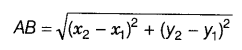

The distance of a point A(x, y) from the origin 0 (0, 0) is given by OA = x2+y2−−−−−−√

Section Formula
The coordinates of the point which divides the joint of (x1, y1) and (x2, y2) in the ratio m : n internally, is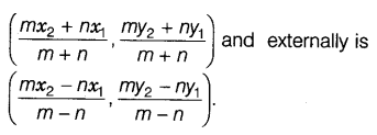

Mid-point of the joint of (x1, y1) and (x2, y2) is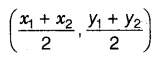

X-axis divides the line segment joining (x1, y1) and (x2, y2) in the ratio -y1 : y2.

Y-axis divides the line segment joining (x1, y1) and (x2, y2) in the ratio -x1 : x2.

The coordinates of the centroid of the triangle whose vertices are (x1, y1), (x2, y2) and (x3, y3) is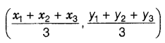

Area of Triangle
The area of the triangle, the coordinates of whose vertices are (x1, y1), (x2, y2)and (x3, y3) is the absolute value of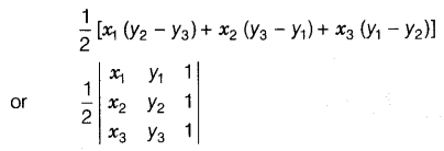

If the points (x1, y1), (x2, y2) and (x3, y3) are collinear, then x1 (y2 – y3) + x2 (y3 – y1) + x3 (y1 – y2) = 0.

Shifting of Origin
Let the origin is shifted to a point O'(h, k). If P(x, y) are coordinates of a point referred to old axes and P'(X, Y) are the coordinates of the same points referred to new axes, then x = X + h, y = Y + k.

Straight Line
Any curve is said to be a straight line if two points are taken on the curve such that every point on the line segment joining any two points on it lies on the curve. General equation of a line is ax + by + c = 0.

Slope or Gradient of Line
The inclination of angle θ to a line with a positive direction of X-axis in the anti-clockwise direction, the tangent of angle θ is said to be slope or gradient of the line and is denoted by m.
i.e. m = tan θ
The slope of a line passing through points P(x1, y1) and Q(x2, y2) is given by

Note: Slope of a line parallel to X-axis is zero and slope of a line parallel to Y-axis is not defined.

Angle between Two Lines
The angle θ between two lines having slope m1 and m2 is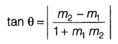

• If two lines are parallel, their slopes are equal i.e. m1 = m2.
• If two lines are perpendicular to each other, then their product of slopes is -1 i.e. m1m2 = -1.

Various Forms of the Equation of a Line
If a line is at a distance k and parallel to X-axis, then the equation of the line is y = ± k.

If a line is parallel to Y-axis at a distance c from Y-axis, then its equation is x = ± c.

Slope-intercept form: The equation of line with slope m and making an intercept c on the y-axis, is y = mx + c.

One point-slope form: The equation of a line which passes through the point (x1, y1) and has the slope of m is given by y – y1 = m (x – x1).

Two points form: The equation of a line passing through the points (x1, y1) and (x2, y2) is given by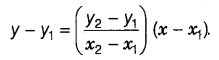

The Intercept form: The equation of a line which cuts off intercepts a and b respectively on the x and y-axes is given by 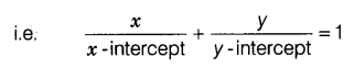xa+yb=1

The normal form: The equation of a straight line upon which the length of the perpendicular from the origin is p and angle made by this perpendicular to the x-axis is α, is given by x cos α + y sin α = p.

General Equation of a Line
Any equation of the form Ax + By + C = 0, where A and B are simultaneously not zero is called the general equation of a line.

Different Forms of Ax + By + C = 0
Slope intercept form: If B ≠ 0, then Ax + By + C = 0 can be written as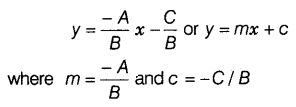

If B = 0, then x = – C / A which is a vertical line, whose slope is not defined and x-intercept is – C/A.

Intercept form If C ≠ 0, then Ax + By + C = 0 can be written as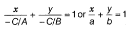

where a = – C / A and b = – C/B
If C = 0, then Ax + By + C = 0 can be written as Ax + By = 0 which is a line passing through origin and therefore has zero intercept on the axes.

Normal form: The normal form of equation Ax + By + C = 0 is x cos α + y sin α = p where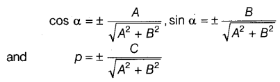

Note: Proper choice of signs to be made so that p should be always positive.

Position of Points is Relative to a Given Line
Let the equation of the given line be ax + by + c = 0 and let the coordinates of the two given points be P(x1, y1) and Q(x2, y2).
The two points are on the same side of the straight line ax + by + c = 0, If ax1 + by1 + c and ax2 + by2 + c have the same sign.

The two points are on the opposite sides of the straight line ax + by + c = 0, If ax1 + by1 + c and ax2 + by2 + c have opposite sign.

Condition of concurrency for three given lines
a1x + b1y + c1 = 0, a2x + b2y + c2 = 0 and a3x + b3y+ c3 = 0 is a3(b1c2 – b2c1) + b3(a2c1 – a1c2) + c3(a1b2 – a2b1) = 0

Point of intersection of two lines
Let equation of lines be ax1 + by1 + c1 = 0 and a2x + b2y + c2 = 0, then their point of intersection is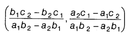

Distance of a Point from a Line
The perpendicular distanced of a point P(x1, y1)from the line Ax + By + C = 0 is given by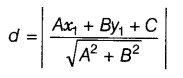

Distance Between Two Parallel Lines
The distance d between two parallel lines y = mx + c1 and y = mx + c2 is given by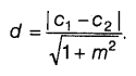

Chapter 11 Conic Sections

Circle
A circle is the set of all points in a plane, which are at a fixed distance from a fixed point in the plane. The fixed point is called the centre of the circle and the distance from centre to any point on the circle is called the radius of the circle.
The equation of a circle with radius r having centre (h, k) is given by (x – h)2 + (y – k)2 = r2.

The general equation of the circle is given by x2 + y2 + 2gx + 2fy + c = 0 , where, g, f and c are constants.

• The centre of the circle is (-g, -f).
• The radius of the circle is r = g2+f2−c−−−−−−−−−√

The general equation of the circle passing through origin is x2 + y2 + 2gx + 2fy = 0.

The parametric equation of the circle x2 + y2 = r2 are given by x = r cos θ, y = r sin θ, where θ is the parametre and the parametric equation of the circle (x – h)2 + (y – k)2 = r2 are given by x = h + r cos θ, y = k + r sin θ.

Note: The general equation of the circle involves three constants which implies that at least three conditions are required to determine a circle uniquely.

Parabola
A parabola is the set of points P whose distances from a fixed point F in the plane are equal to their distance from a fixed line l in the plane. The fixed point F is called focus and the fixed line l is the directrix of the parabola.

Main Facts About the Parabola

Forms of parabola	y2= 4ax	y2 = -4ax	x2 = 4ay	x2 = -4ay
Axis of parabola	y = 0	y = 0	x = 0	x = 0
Directrix of parabola	x = -a	x = a	y = -a	y = a
Vertex	(0, 0)	(0, 0)	(0, 0)	(0, 0)
Focus	(a, 0)	(-a, 0)	(0, a)	(0, -a)
Length of latus rectum	4a	4a	4a	4a
Focal length	|x + a|	|x – a|	|y + a|	|y – a|

Ellipse
An ellipse is the set of all points in a plane such that the sum of whose distances from two fixed points is constant.
or
An ellipse is the set of all points in the plane whose distances from a fixed point in the plane bears a constant ratio, less than to their distance from a fixed point in the plane. The fixed point is called focus, the fixed line a directrix and the constant ratio(e) the eccentricity of the ellipse. We have two standard forms of ellipse i.e.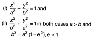

Main Facts about the Ellipse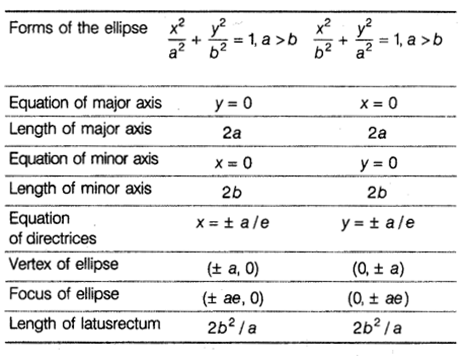

Hyperbola
A hyperbola is the locus of a point in a plane which moves in such a way that the ratio of its distance from a fixed point in the same plane to its distance from a fixed line is always constant which is always greater than unity. The fixed point is called the focus, the fixed line is called the directrix and the constant ratio, generally denoted bye, is known as the eccentricity of the hyperbola.
We have two standard forms of hyperbola i.e.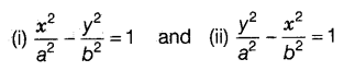

Main Facts About Hyperbola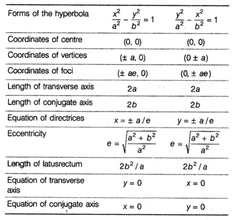

Chapter 12 Introduction to Three Dimensional Geometry

Coordinate Axes
In three dimensions, the coordinate axes of a rectangular cartesian coordinate system are three mutually perpendicular lines. These axes are called the X, Y and Z axes.

Coordinate Planes
The three planes determined by the pair of axes are the coordinate planes. These planes are called XY, YZ and ZX plane and they divide the space into eight regions known as octants.

Coordinates of a Point in Space
The coordinates of a point in the space are the perpendicular distances from P on three mutually perpendicular coordinate planes YZ, ZX, and XY respectively. The coordinates of a point P are written in the form of triplet like (x, y, z).
The coordinates of any point on

• X-axis is of the form (x, 0,0)
• Y-axis is of the form (0, y, 0)
• Z-axis is of the form (0, 0, z)
• XY-plane are of the form (x, y, 0)
• YZ-plane is of the form (0, y, z)
• ZX-plane are of the form (x, 0, z)

Distance Formula
The distance between two points P(x1, y1, z1) and Q(x2, y2, z2) is given by

The distance of a point P(x, y, z) from the origin O(0, 0, 0) is given by
OP = x2+y2+z2−−−−−−−−−−√

Section Formula
The coordinates of the point R which divides the line segment joining two points P(x1, y1, z1) and Q(x2, y2, z2) internally or externally in the ratio m : n are given by

The coordinates of the mid-point of the line segment joining two points P(x1, y1, z1) and Q(x2, y2, z2) are

The coordinates of the centroid of the triangle, whose vertices are (x1, y1, z1), (x2, y2, z2) and (x3, y3, z3) are

Chapter 13 Limits and Derivatives

Limit
Let y = f(x) be a function of x. If at x = a, f(x) takes indeterminate form, then we consider the values of the function which is very near to a. If these value tend to a definite unique number as x tends to a, then the unique number so obtained is called the limit of f(x) at x = a and we write it as limx→af(x).

Left Hand and Right-Hand Limits
If values of the function at the point which are very near to a on the left tends to a definite unique number as x tends to a, then the unique number so obtained is called the left-hand limit of f(x) at x = a, we write it as

Existence of Limit

Some Properties of Limits
Let f and g be two functions such that both limx→af(x) and lim limx→ag(x) exists, then

Some Standard Limits

Derivatives
Suppose f is a real-valued function, then

Fundamental Derivative Rules of Function
Let f and g be two functions such that their derivatives are defined in a common domain, then

Some Standard Derivatives

Chapter 14 Mathematical Reasoning

Statements
A statement is a sentence which is either true or false, but not both simultaneously.

Note:
No sentence can be called a statement if

• It is an exclamation.
• It is an order or request.
• It is a question.

Simple Statements
A statement is called simple if it cannot be broken down into two or more statements.

Compound Statements
A compound statement is the one which is made up of two or more simple statement.

Connectives
The words which combine or change simple statements to form new statements or compound statements are called connectives.

Conjunction
If two simple statements p and q are connected by the word ‘and’, then the resulting compound statement “p and q” is called a conjunction of p and q is written in symbolic form as “p ∧ q”.

Note:

• The statement p ∧ q has the truth value T (true) whenever both p and q have the truth value T.
• The statement p ∧ q has the truth value F (false) whenever either p or q or both have the truth value F.

Disjunction
If two simple statements p and q are connected by the word ‘or’, then the resulting compound statement “p or q” is called disjunction of p and q and is written in symbolic form as “p ∨ q”.

Note:

• The statement p ∨ q has the truth value F whenever both p and q have the truth value F.
• The statement p ∨ q has the truth value T whenever either p or q or both have the truth value T.

Negation
An assertion that a statement fails or denial of a statement is called the negation of the statement. The negation of a statement p in symbolic form is written as “~p”.

Note:

• ~p has truth value T whenever p has truth value F.
• ~p has truth value F whenever p has truth value T.

Negation of Conjunction
The negation of a conjunction p ∧ q is the disjunction of the negation of p and the negation of q.
Equivalently we write ~ (p ∧ q) = ~p ∨ ~q.

Negation of Disjunction
The negation of a disjunction p v q is the conjunction of negation of p and the negation of q.
Equivalently, we write ~(p ∨ q) = ~p ∧ ~q.

Negation of Negation
Negation of negation of a statement is the statement itself.
Equivalently, we write ~(~p) = p

The Conditional Statement
If p and q are any two statements, then the compound statement “if p then g” formed by joining p and q by a connective ‘if-then’ is called a conditional statement or an implication and is written in symbolically p → q or p ⇒ q, here p is called hypothesis (or antecedent) and q is called conclusion (or consequent) of the conditional statement (p ⇒ q).

Contrapositive of Conditional Statement
The statement “(~q) → (~p) ” is called the contrapositive of the statement p → q.

Converse of a Conditional Statement
The conditional statement “q → p” is called the converse of the conditional statement “p → q”.

Inverse of Conditional Statement
The Conditional statement “q → p” is called inverse of p → q.

The Biconditional Statement
If two statements p and q are connected by the connective ‘if and only if’, then the resulting compound statement “p if and only if q” is called biconditional of p and q and is written in symbolic form as p ⇔ q.

Quantifier
(i) For all or for every is called universal quantifier.
(ii) There exists is called existential quantifier.

Validity of Statements
A statement is said to valid or invalid according to as it is true or false.
If p and q are two mathematical statements, then the statement
(i) “p and q” is true if both p and q are true.
(ii) “p or g” is true if p is false
⇒ q is true orq is false ⇒ p is true.
(iii) “If p, then q” is true p is true ⇒ q is true
or
q is false
⇒ p is false
or
p is true and q is false less us to a contradiction,
(iv) “p if and only if q” is true, if
(a) p is true ⇒ q is true and
(b) q is true ⇒ p is true.

Chapter 15 Statistics

Measure of Dispersion
The dispersion is the measure of variations in the values of the variable. It measures the degree of scatteredness of the observation in a distribution around the central value.

Range
The measure of dispersion which is easiest to understand and easiest to calculate is the range.
Range is defined as the difference between two extreme observation of the distribution.
Range of distribution = Largest observation – Smallest observation.

Mean Deviation
Mean deviation for ungrouped data
For n observations x1, x2, x3,…, xn, the mean deviation about their mean x¯ is given by

Mean deviation about their median M is given by

Mean deviation for discrete frequency distribution
Let the given data consist of discrete observations x1, x2, x3,……., xn occurring with frequencies f1, f2, f3,……., fn respectively in case

Mean deviation about their Median M is given by

Mean deviation for continuous frequency distribution

where xi are the mid-points of the classes, x¯ and M are respectively, the mean and median of the distribution.

Variance
Variance is the arithmetic mean of the square of the deviation about mean x¯.
Let x1, x2, ……xn be n observations with x¯ as the mean, then the variance denoted by σ2, is given by

Standard deviation
If σ2 is the variance, then σ is called the standard deviation is given by

Standard deviation of a discrete frequency distribution is given by

Standard deviation of a continuous frequency distribution is given by

Coefficient of Variation
In order to compare two or more frequency distributions, we compare their coefficient of variations. The coefficient of variation is defined as

Note: The distribution having a greater coefficient of variation has more variability around the central value, then the distribution having a smaller value of the coefficient 0f variation.

Chapter 16 Probability

Random Experiment
An experiment whose outcomes cannot be predicted or determined in advance is called a random experiment.

Outcome
A possible result of a random experiment is called its outcome.

Sample Space
A sample space is the set of all possible outcomes of an experiment.

Events
An event is a subset of a sample space associated with a random experiment.

Types of Events
Impossible and sure events: The empty set Φ and the sample space S describes events. Intact Φ is called the impossible event and S i.e. whole sample space is called sure event.

Simple or elementary event: Each outcome of a random experiment is called an elementary event.

Compound events: If an event has more than one outcome is called compound events.

Complementary events: Given an event A, the complement of A is the event consisting of all sample space outcomes that do not correspond to the occurrence of A.

Mutually Exclusive Events
Two events A and B of a sample space S are mutually exclusive if the occurrence of any one of them excludes the occurrence of the other event. Hence, the two events A and B cannot occur simultaneously and thus P(A ∩ B) = 0.

Exhaustive Events
If E1, E2,…….., En are n events of a sample space S and if E1 ∪ E2 ∪ E3 ∪………. ∪ En = S, then E1, E2,……… E3 are called exhaustive events.

Mutually Exclusive and Exhaustive Events
If E1, E2,…… En are n events of a sample space S and if
Ei ∩ Ej = Φ for every i ≠ j i.e. Ei and Ej are pairwise disjoint and E1 ∪ E2 ∪ E3 ∪………. ∪ En = S, then the events
E1, E2,………, En are called mutually exclusive and exhaustive events.

Probability Function
Let S = (w1, w2,…… wn) be the sample space associated with a random experiment. Then, a function p which assigns every event A ⊂ S to a unique non-negative real number P(A) is called the probability function.
It follows the axioms hold

• 0 ≤ P(wi) ≤ 1 for each Wi ∈ S
• P(S) = 1 i.e. P(w1) + P(w2) + P(w3) + … + P(wn) = 1
• P(A) = ΣP(wi) for any event A containing elementary event wi.

Probability of an Event
If there are n elementary events associated with a random experiment and m of them are favorable to an event A, then the probability of occurrence of A is defined as

The odd in favour of occurrence of the event A are defined by m : (n – m).
The odd against the occurrence of A are defined by n – m : m.
The probability of non-occurrence of A is given by P(A¯) = 1 – P(A).

Addition Rule of Probabilities
If A and B are two events associated with a random experiment, then
P(A ∪ B) = P(A) + P(B) – P(A ∩ B)
Similarly, for three events A, B, and C, we have
P(A ∪ B ∪ C) = P(A) + P(B) + P(C) – P(A ∩ B) – P(A ∩ C) – P(B ∩ C) + P(A ∩ B ∩ C)

Note: If A andB are mutually exclusive events, then
P(A ∪ B) = P(A) + P(B)